Interpretation of Data

Figure 5: Chart for interpretation of emission mechanism from the spectrum distribution

38#38

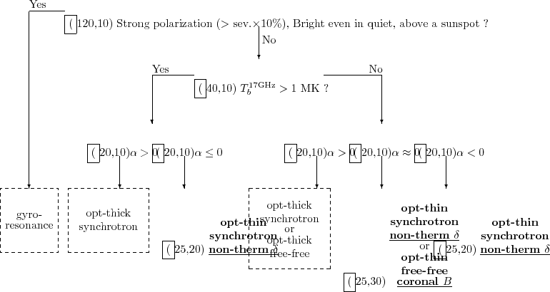
The interpretation is done by using the chart in Figure 5. Physical information can be obtained when the emission is by "optically-thin gyrosynchrotron" or by "optically-thin free-free". We can derive the variable using the Dulk's (1985) models.

In case "optically-thin gyrosynchrotron" emission, we obtain power-law index of the non-thermal electrons. Here we assume the distribution function of electrons to be

39#39

where 18#18 is electron energy (keV), 19#19 is number of electrons (particles) that has larger energy than 18#18. This distribution is described with parameters 20#20, 21#21, and 22#22. But it is usual to use 23#23 instead of 22#22. And we fix 24#24 after Dulk (1985). If we find the emission to be "optically-thin gyrosynchrotron", we will obtain 20#20 from 14#14 by

40#40

In case "optically-thin free-free" emission, we obtain line-of-sight component of coronal magnetic field. From the circular polarization degree 13#13,

41#41

For example, figure 4 can be interpreted as follows: First, the strong polarized source at 42#42 is by gyroresonance. It may be confirmed by comparing the image with optical magnetogram to see if there is a sunspot. Next, the area inside the contour line of 3#3 is emitting by optically-thin gyrosynchrotron. Non-thermal power-law index 20#20 is obtained from 14#14 immediately and we see that the emission from two-sides of the loop structure is 'softer' than that of the top. Next is for the area where 43#43. Around 44#44, it is hard to judge if it is 'optically-thin gyrosynchrotron' or "optically-thin free-free" because 45#45. If it is bright in soft X-ray it may be free-free emission. In this case, line-of-sight component of coronal magnetic field is obtained. Since the other area has 46#46, it is optically thick and no information can be obtained.