How to use the NoRP Python library on SunPy
9 November 2026
M. Shimojo
Contents
- Preparation
- Obtain and plot the long-term (>a day) data
- Obtain and plot the short-term (<a day) data
- Fitting a spectrum of a solar flare
1. Preparation
The following procedure can be used on the SunPy environment. Hence, at first, SunPy is installed. The install manual of SunPy is described in the following SunPy website.
Installation, The Sunpy tutorial
After the installation, download the following the python script.
norp_fits.py
Then, put the script on your working directory,
or add the path that the script is located using the following commands in the your script.
Let's do analyzing NoRP data on SunPy !!
2. Obtain and plot the Long-Term (>a day) data
2.1. Long-term dataset of Toyokawa/Nobeyama Radio Polarimeters
Continuous monitoring of solar microwave fluxes began in the 1950s at the Toyokawa campus of Nagoya University and has been continued at the Nobeyama campus of the National Astronomical Observatory of Japan. As a result, the observation record now spans more than 70 years. Because the radio telescopes were originally designed to observe solar radio bursts, the microwave flux data obtained by the Nobeyama Radio Polarimeters (NoRP) have a high temporal resolution of 0.1 s. While this resolution is well suited for studies of rapid solar radio phenomena, it is unnecessarily high for investigations of long-term variations in solar microwave fluxes on timescales of a day or longer. To support investigations of the long-term variability of solar microwave fluxes, we provide text files of tables of daily fluxes at 1, 2, 3.75, and 9.4 GHz, along with the corresponding CSV files, via an online repository. Here, the term "daily flux" denotes the solar microwave flux derived from observations obtained in the absence of major solar flares. Because the flux values are calcurated through manual inspection, the dataset has been carefully curated to exclude data affected by poor weather conditions, instrumental malfunctions, radio-frequency interference (RFI), and other observational artifacts. In the following section, we demonstrate the NoRP long-term datasetuse within the SunPy framework.
2.2 Obtain the long-term NoRP dataset from the internet and plot it.
Import the necessary Python libraries, and the TimeSeries object of the Long-Term NoRP data (daily_ts) is createdas using "NoRPDailyTimeSerie" as follows.
"NoRPDailyTimeSeries" automatically retrieves the CSV files from the online archive and creates a TimeSeries object. The NoRP long-term dataset is available in two versions. One contains the observed solar microwave fluxes at Earth, while the other contains fluxes normalized to a distance of 1 AU from the Sun. The latter dataset is corrected for variations in the Sun-Earth distance. For studies of intrinsic solar variability, the corrected dataset should be used by setting the option "au_corr=True". In contrast, if the objective is to investigate the influence of solar activity on Earth's upper atmosphere, the uncorrected dataset should be used by setting "au_corr=False".
Once created, the TimeSeries object returned by NoRPDailyTimeSeries can be analyzed and visualized using the standard SunPy TimeSeries interface. The following example plots the data over the entire observation period.
st = daily_ts.time[0].to_datetime()
ed = daily_ts.time[-1].to_datetime()
fig, ax = plt.subplots()
daily_ts.plot(axes=ax,columns=['9.4 GHz', '3.75 GHz', '2 GHz','1 GHz'],
marker='.', linestyle='None', ms=0.5)
plt.legend(loc='upper left', fontsize=5)
plt.xlabel(f'Year [{st.strftime("%Y/%m/%d")} -- {ed.strftime("%Y/%m/%d")}]')
plt.ylabel('Flux Density@ 1 AU [Jy = $10^{-4}$ SFU]')
plt.show()
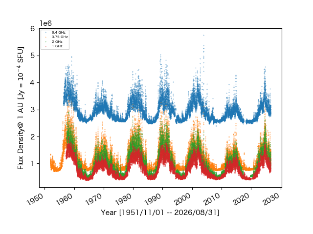 Caution: Due to no "SFU" unit in AstroPy, the unit of the fluxes is "Jy".
When you want to plot a part of the data,
tr = TimeRange('1996-06-01 00:00', '2018-06-01 00:00')
daily_ts12 = daily_ts.truncate(tr)

fig, ax = plt.subplots()
daily_ts12.plot(axes=ax,columns=['9.4 GHz', '3.75 GHz', '2 GHz','1 GHz'],
                marker='.', linestyle='None', ms=0.5)
plt.legend(loc='upper left', fontsize=10)
plt.ylabel('Flux Density@ 1 AU [Jy = $10^{-4}$ SFU]')
plt.show()
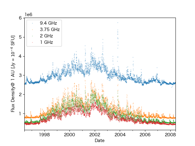
3. Obtain and plot the short-term (<a day) data
3.1 The data files of the NoRP observations
The raw NoRP data are stored in a proprietary format that can be read only with the Interactive Data Language (IDL) and the SolarSoftWare (SSW) package. Each raw data file contains observations acquired during a single day. The daily observing period varies with season. Because the IDL/SSW environment is not commonly used outside the solar physics community, we provide NoRP data in FITS format through our website. Each FITS file contains both the raw observational data and the calibrated microwave fluxes obtained by NoRP for a given day. The SunPy interface described below automatically downloads the corresponding FITS file and creates a TimeSeries object from the calibrated microwave fluxes contained in the file.
3.2 Obtain the NoRP FITS files from the internet and plot it.
At first, import the necessary Python libraries, and set the time period and observing frequencies that you want to analyze. Then, search and download the FITS file.
#-------------import the librarie--------------------------------
from sunpy.net import attrs as a
from sunpy.net import Fido
from norp_fits import NoRPTimeSeries
import matplotlib.pyplot as plt
from datetime import datetime, timezone

#-------------parameter setup--------------------------------
st = '2014-12-19 20:00:00.000' # start time of reading data
et = '2014-12-20 09:00:00.000' # end time of reading data

getFreq = [1, 1, 1, 1, 1, 1, 0]
# the observing frequency (1, 2, 3.75, 9.4, 14, 35, 80 GHz from left)
# In the above case, we do not read 80 GHz data.

#-------------Search and download the FITS file --------------------------------
results = Fido.search(a.Time(st,et), a.Instrument.norp)
print(results.show())
filenames = Fido.fetch(results, path='.')
"Fido.search" and "Fido.fetch" shows the following message and puts the FITS file in your working directory.
Results from 1 Provider:

1 Results from the NoRPClient:
Source: https://solar.nro.nao.ac.jp/norp/index.html

       Start Time               End Time        Instrument   Physobs    Source Provider                               url
----------------------- ----------------------- ---------- ------------ ------ -------- ----------------------------------------------------------------
2014-12-19T22:09:59.072 2014-12-20T07:09:54.856       NORP flux density    SSO     NAOJ https://solar.nro.nao.ac.jp/norp/fits/2014/12/norp141220.fits.gz


Files Downloaded: 100%|███████████████████████████████████| 1/1 [00:00<00:00, 22.57file/s]
Then, we create the TimeSeries object from the FITS file and plot it.
#-------------Creat TimeSeries object and plot----------------------------
ts = NoRPTimeSeries(filenames[0], getFreq = getFreq,
                    Stokes = "I")
#In the case, we create the TimeSeries object only from Stokes-I data.
# If you want Stokes-V data, set Stokes = "V" and Stokes = "IV"

fig, ax = plt.subplots()
ts.plot(axes=ax, columns=['1GHz-I', '2GHz-I', '3.75GHz-I', '9.4GHz-I','17GHz-I', '35GHz-I'],
        marker='.', ms=1, linewidth=0)
plt.ylabel('Flux Density [Jy = $10^{-4}$ SFU]')
plt.show()
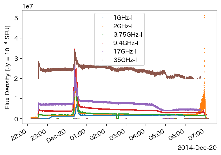
Caution1: Due to no "SFU" unit in AstroPy, the unit of the fluxes is "Jy".
Caution2: "NoRPTimeSeries" can reads one FITS file only at once.
Once created, the TimeSeries object returned by NoRPTimeSeries can be analyzed and visualized using the standard SunPy TimeSeries interface.
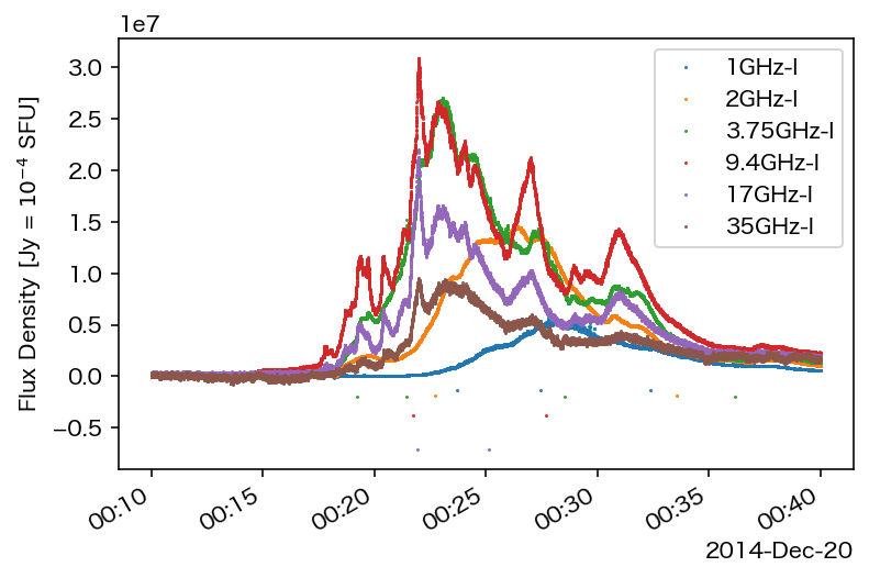
On the day, a flare occurred around 00:20UT. So, we make a TimeSeries object only from the flare period and plot it.
#---------- make TS only for flate and plot it --------------------
fst = '2014-12-20 00:10:00.000' # start time of reading data for the flare
fet = '2014-12-20 00:40:00.000' # end time of reading data for the flare

tsf = NoRPTimeSeries(filenames[0], getFreq = getFreq,
                    timeRange = [fst,fet], Stokes = "I")

fig, ax = plt.subplots()
tsf.plot(axes=ax, columns=['1GHz-I', '2GHz-I', '3.75GHz-I', '9.4GHz-I','17GHz-I', '35GHz-I'],
        marker='.', ms=1, linewidth=0)
plt.ylabel('Flux Density [Jy = $10^{-4}$ SFU]')
plt.show()
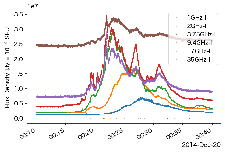
When you want to subtract the background,
fbg = '2014-12-20 00:13:00.000' # Time of background

tsf = NoRPTimeSeries(filenames[0], getFreq = getFreq,
                    timeRange = [fst,fet], bgtime=fbg, Stokes = "I")

fig, ax = plt.subplots()
tsf.plot(axes=ax, columns=['1GHz-I', '2GHz-I', '3.75GHz-I', '9.4GHz-I','17GHz-I', '35GHz-I'],
        marker='.', ms=1, linewidth=0)
plt.ylabel('Flux Density [Jy = $10^{-4}$ SFU]')
plt.show()
4. Fitting a spectrum of a solar flare
4.1 Model microwave spectrum of solar flares
During a solar flare, the solar radio flux can increase significantly. In the microwave range, this enhancement is primarily produced by gyrosynchrotron emission from high-energy electrons accelerated during the flare. In the optically thin regime, the microwave spectrum can be described by a power-law function, and its spectral index provides important information on the energy distribution of the high-energy electrons. However, the microwave emission observed during solar flares, particularly within the NoRP frequency range, generally consists of contributions from both optically thick and optically thin regions. Therefore, deriving the power-law index of the optically thin component requires fitting the observed spectrum with a spectral model, such as that given below, and subsequently estimating the spectral index from the fitted parameters.

Here are 4 fitting parameters: νb is turn-over frequency,
F̂ν is turn-over flux density, αtk is power index
of low frequency side (optically thick side) and αtn is power index of high frequency side (optically thin
side), respectively.
4.2 Preparation for spectrum fitting
Spectral fitting is performed using the Markov Chain Monte Carlo (MCMC) technique. The following library packages for Python are required:
Once the packages have been installed, download the following script and save it in your working directory.
norp_mcmc_fit.py
4.3 Obtain the NoRP data and extract the flare spectrum at the interest time range
At first, import the necessary Python libraries, and set the time period and observing frequencies that you want to analyze. Then, search and download the FITS file.
#-------------import the librarie--------------------------------
from sunpy.net import attrs as a
from sunpy.net import Fido
from norp_fits import NoRPTimeSeries
import matplotlib.pyplot as plt
from datetime import datetime, timezone
import numpy as np
from norp_mcmc_fit import norp_mcmc_fit

#-------------parameter setup--------------------------------
fst = '2014-12-20 00:10:00.000' # start time of reading data for the flare
fet = '2014-12-20 00:40:00.000' # end time of reading data for the flare
fbg = '2014-12-20 00:13:00.000' # background
getFreq = [1, 1, 1, 1, 1, 1, 0]
# the observing frequency (1, 2, 3.75, 9.4, 14, 35, 80 GHz from left)
# In the above case, we do not read 80 GHz data.

#-------------Search and download the FITS file--------------------------------
results = Fido.search(a.Time(fst,fet), a.Instrument.norp)
print(results.show())
filenames = Fido.fetch(results, path='.')
Next, we create a TimeSeries object from the FITS file. The native time resolution of the NoRP data is 0.1 s. In many cases, this temporal resolution is higher than necessary for spectral fitting, resulting in a relatively low signal-to-noise ratio (S/N) for individual measurements. To improve the S/N ratio, the data are averaged over a specified time interval. In the following example, the data are integrated over 2 seconds, corresponding to 20 consecutive data points. Of course, we need to subtract the background
#---------- make TS only for flate --------------------
tsf = NoRPTimeSeries(filenames[0], getFreq = getFreq,
                    timeRange = [fst,fet], Stokes = "I",
                    bgtime=fbg, intg=2)
To extract the flare spectrum over a specific time interval, we first obtain the time array from the TimeSeries object and identify the indices corresponding to the time range of interest. The spectral data within that interval are then extracted from the TimeSeries object
#---------------extract the flare spectrum at the intreste time ----------------
tgttime = '2014-12-20 00:22:02.000' # target time for spectrum fitting.
tim = list(tsf.time.datetime)
cnt = 0
while cnt <= len(tim)-1:
tim[cnt] = tim[cnt].replace(tzinfo = timezone.utc)
cnt += 1
tgti = datetime.fromisoformat(tgttime)
tgti = tgti.replace(tzinfo = timezone.utc)
tgt_mindiff = min(tim, key=lambda t: abs(t - tgti))
tgtInd = tim.index(tgt_mindiff)
spec0 = tsf.to_array()[tgtInd]/1e4 #Convert unit from "Jy" to "SFU"
#Error is 3% of Fluxes.
spec_err0 = np.sqrt(2*(spec0*0.03)**2) #Assuming that the error of the observation is 3%.
obsfreq0 = [1, 2, 3.75, 9.4, 17, 35, 80]
#--------plot time profile of the flare and the spectgrum at the intreste time
fig = plt.figure(figsize=(6.4*2, 4.8*1))
ax1 = fig.add_subplot(1, 2, 1)
ax2 = fig.add_subplot(1, 2, 2)
tsf.plot(columns=['1GHz-I', '2GHz-I', '3.75GHz-I', '9.4GHz-I','17GHz-I', '35GHz-I'],
marker='.', ms=5, linewidth=0,axes=ax1)
ax1.set_xlabel('Time')
ax1.set_ylabel('Solar Fluxes Stokes-I [Jy]')
ax1.axvline(x=tim[tgtInd], color="black", linestyle="--")
ax1.legend(ncol=1, fontsize=10)
ax1.minorticks_on()
ax1.set_ylim([-0.1e7,3e7])
ax2.plot(obsfreq0, spec0, marker='.', ms=10, linewidth=0)
ax2.errorbar(obsfreq0, spec0, yerr=spec_err0, fmt=".k", capsize=0)
ax2.set_title(str(tim[tgtInd]))
ax2.set_xlabel('Frequency [GHz]')
ax2.set_ylabel('Solar Fluxes Stokes-I [SFU]')
ax2.set_xscale('log')
ax2.set_yscale('log')
plt.show()
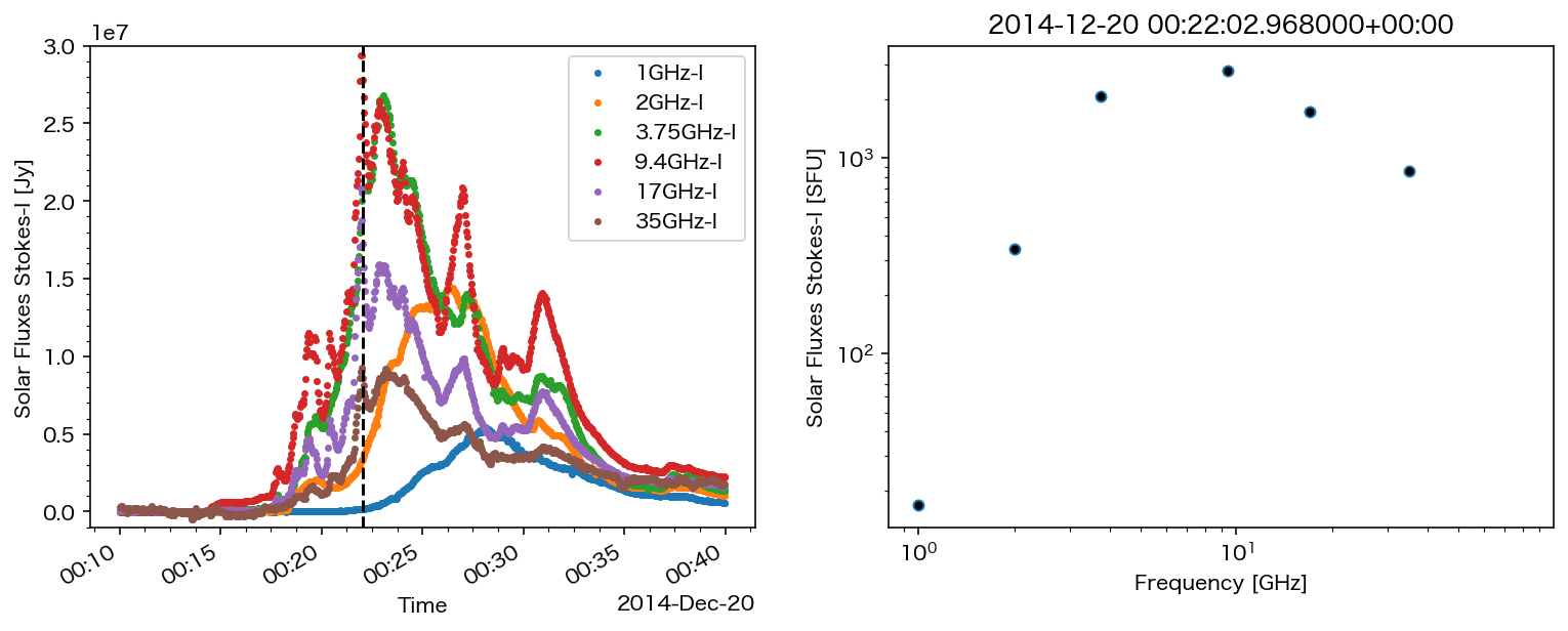 The black dashed vertical line indicates the intreste time.
The unit of the fluxes is converted from "Jy" to "SFU" due to avoiding the unstable in the fitting process.
4.4 Spectrum fitting and plot the results
At first, delete the data not used for fitting from the array.
Then, the fititng is started.
sol, ferr, fitres = norp_mcmc_fit(obsfreq, spec, spec_err)
# Main subroutine for the mcmc fitting.
The subroutine plots the following and prints out the first guess
The first guess for 1st fitting is not sutable in most cases. Hence, the fitting is not converged as shown in the above plot. In the plot, a0, a1, a3 are F̂ν, αtk, -1 x (αtn - αtk), respectively. a2 is F̂νa3. The fitting using the result of the first fitting process is restarted automatically.
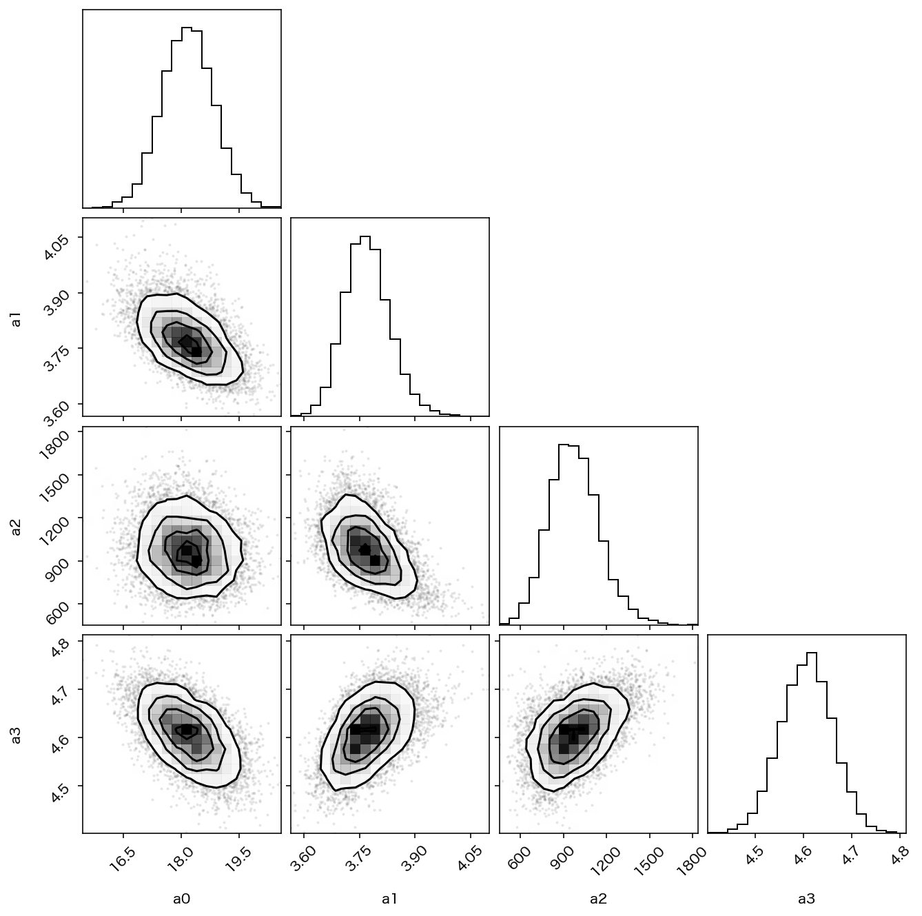
The fitting process is continued until when the fitting is converged or finishing 10 times of the process. The above plot shows the parameter evolutions in the itaration process when the fittig is converged. And then, the below plots are shown.
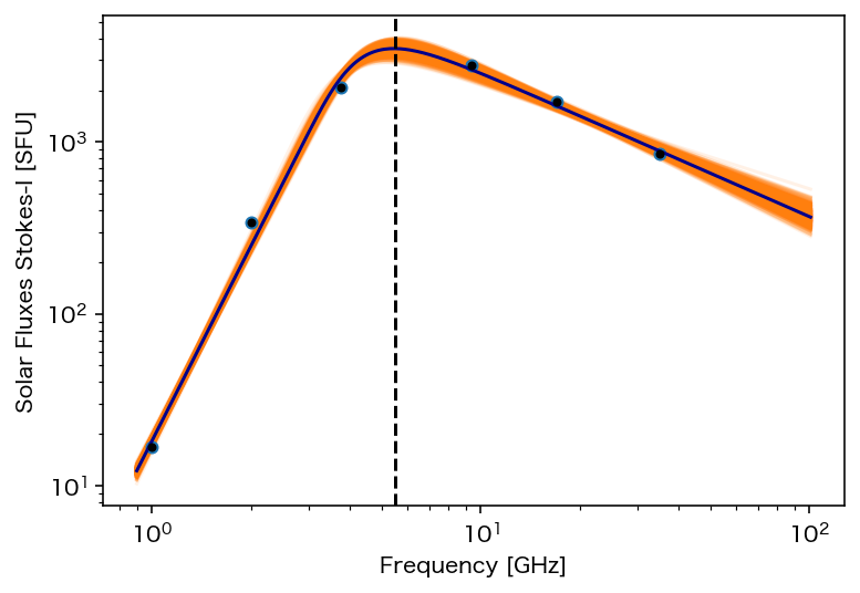
The blue line is the result of the fitting, and the vertical dashed lines indicates the turn-over frequency. The orange lines shows the range of one-sigma error in the fitting.
The process outputs three following values. "sol" includes the result of the fitting parameters (a0,a1,a2,a3), "ferr" inlcudes the one-sigma error of the parameters calculate from the distributions shown in the corner plot, and "fitres" includes αtn, the error of αtn and νb. When the fitting is not converged, only "sol" includes the values.
Then, we plot the results, as follows.
fig = plt.figure(figsize=(6.4*2, 4.8*1))
ax1 = fig.add_subplot(1, 2, 1)
ax2 = fig.add_subplot(1, 2, 2)
tsf.plot(columns=['1GHz-I', '2GHz-I', '3.75GHz-I', '9.4GHz-I',
   	    	     '17GHz-I', '35GHz-I'],
   	    marker='.', ms=5, linewidth=0,axes=ax1)
ax1.set_xlabel('Time')
ax1.set_ylabel('Solar Fluxes Stokes-I [Jy]')
ax1.axvline(x=tim[tgtInd], color="black", linestyle="--")
ax1.legend(ncol=1, fontsize=10)
ax1.minorticks_on()
ax1.set_ylim([-0.1e7,3e7])
xx = (np.arange(1000)*0.1+0.9)
yy = sol[0] * xx**sol[1] * (1 - np.exp(-1 * sol[2] * xx ** (-1 * sol[3])))
ax2.plot(obsfreq, spec, marker='.', ms=10, linewidth=0)
ax2.plot(xx, yy)
ax2.errorbar(obsfreq, spec, yerr=spec_err, fmt=".k", capsize=0)
ax2.set_title('X1.8 flare at '+str(tim[tgtInd]))
ax2.set_xlabel('Frequency [GHz]')
ax2.set_ylabel('Solar Fluxes Stokes-I [SFU]')
ax2.axvline(fitres[2], color="black", linestyle="--")
ax2.set_xscale('log')
ax2.set_yscale('log')
plt.show()
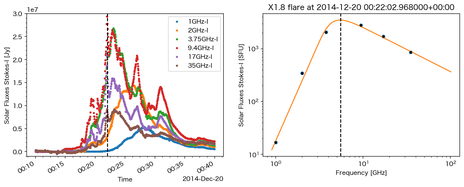
Then, print out the values of the power-law indexes and turn-over frequency.
print("==============================================")
print("Result of Fitting")
print("Power-law Index (Optically Thick part): {0:.2f}".format(sol[1])+" +/-{0:.2f}".format((ferr[3]-ferr[2])/2.))
print("Power-law Index (Optically Thin part): {0:.2f}".format(fitres[0])+" +/-{0:.2f}".format(fitres[1]))
print("Turn-over Frequency: {0:.2f}".format(fitres[2])+" GHz")
print("==============================================")
==============================================
Result of Fitting
Power-law Index (Optically Thick part): 3.77 +/-0.06
Power-law Index (Optically Thin part): 0.84 +/-0.08
Turn-over Frequency: 5.50 GHz
==============================================
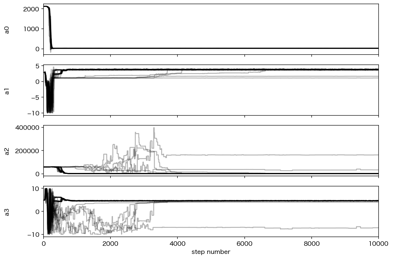 The progress of the first fitting with the not-suitable guess.
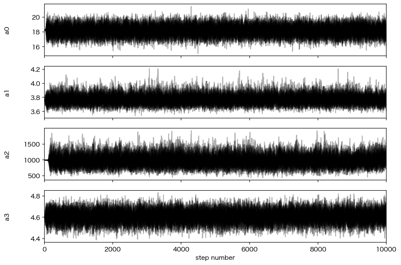 The progress of the fitting with the suitable guess.
 The plot of the fitting result.