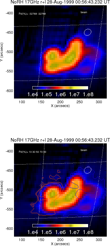
Next, plot the images. We use a FITS file ipa990828_005642.
This file contains "an image of partial Sun of 17 GHz (R+L) component
at 00:56:42 UT on Aug 28, 1999". To read
IDL> file='./ipa990828_005642' ![]() CR
CR![]()
IDL> norh_rd_img,file,indexa,dataa ![]() CR
CR![]()
IDL> stepper,dataa,norh_get_info(indexa) ![]() CR
CR![]()
IDL> norh_grid,indexa ![]() CR
CR![]()
Easy plot is (Fig 2)
IDL> norh_plot,indexa,dataa ![]() CR
CR![]()
The unit of data is brightness temperature (K). Solar north is up.
For preparing to overplot with other instrumental data, change the
data format to SolarSoftware map.
IDL> norh_index2map,indexa,dataa,mapa ![]() CR
CR![]()
IDL> plot_map,mapa,/cont,/grid ![]() CR
CR![]()
IDL> beam=norh_beam(indexa,xbeam=xbeam) ![]() CR
CR![]()
IDL> contour,beam,!x.crange(0)+xbeam,!y.crange(0)+xbeam,/over,levels=[0.5]
![]() CR
CR![]()